
A gentle introduction to Spice
22 Nov 2014SPICE is an indispensable tool for simulating integrated circuits. Here, however, we would look at the SPICE as a tool for developing embedded electronics. Simulation always brings in some sanity and confidence in the head of the designer. That is precisely the goal of this tutorial series. Sanity.
SPICE provides 4 basic analysis
- OP: (Operating Point analysis) Determine the steady state operating point of the circuit under simulation. Example, this analysis helps determine the quiescent voltage and current of say, a transistor amplifier.
- DC: In this analysis, the source input voltage of a circuit is varied over a range (say from 1V to 5V) and the behaviour of the circuit is observed over this range. Example, this can help determine the range over which a transistor remains in linear mode.
- AC: The frequency of a voltage source is varied over a range of frequencies and behaviour of the circuit is observed over this frequency range. Example, this can help plot the frequency response of a RC filter
- Transient: This analysis helps observe the behaviour of a circuit over time. Example, plotting the response of a circuit to a pulse input
We would go over each of the above mentioned analysis with simple examples.
Introducing OP and DC
Let’s start with the simplest form of analysis: Operating Point Analysis. SPICE performs this analysis before performing any other analysis.
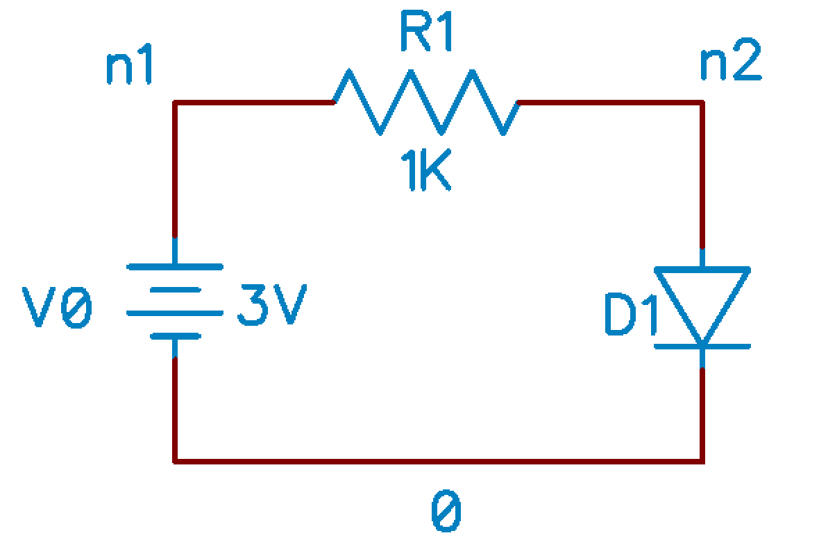
Resistor and Diode

R1 n1 n2 1K
D1 n2 0
V0 n1 0 DC 3V
.end
Save this file as ckt1.cir. SPICE files are conventionally stored with the .cir extension. Names of nodes in the circuit start with n.
First line of the file is the Title Line, and the last line of the file should be .end. The syntax for describing the basic components is as shown
| Component | Syntax |
|---|---|
| Resistor | R<name> <node 1> <node 2> value |
| Diode | D<name> <anode> <cathode> <model name> |
| Voltage source | V<name> <pos> <neg> DC <value> AC <value> |
| Inductor | L<name> <node 1> <node 2> value |
| Capacitor | C<name> <node 1> <node 2> value |
SPICE understands that 1K is one thousand. Shown below is a description of the units SPICE understands.
| SPICE Symbol | Value in Scientific Notation |
|---|---|
| T | 1E12 |
| G | 1E9 |
| MEG | 1E6 |
| K | 1E3 |
| M | 1E-3 |
| U | 1E-6 |
| N | 1E-9 |
| P | 1E-12 |
| F | 1E-15 |
Now, fire up ngspice in a terminal and execute the following
ngspice -> source ckt1.cir
ngspice -> op
ngspice -> show d1
op does the operating point analysis of the circuit; show d1 displays the operating point of D_1.
ngspice -> show D1

Diode: Junction Diode model
device                    d1
model                     D
vd                        0.676901
id                        0.00232313
gd                        0.0898203
cd                        0
Similarily, you can try out
ngspice -> show r1
ngspice -> show v0
ngspice -> show
The last show command displays operating point of all circuit elements in the circuit. To perform a DC sweep analysis, run the following
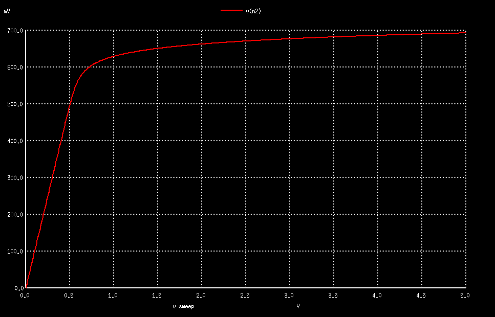
ngspice -> dc v0 0V 5V 0.01V
ngspice -> plot v(n2)
The syntax for describing DC analysis is dc v<name> <vstart> <vstop> <vstep>.This sweeps the voltage source from 0V to 5V in steps of 0.01V & plots the voltage at n2 for this sweep. This results in the plot shown below
While you are at it, try running the following
ngspice -> plot i(v0)
ngspice -> plot i(r1)
ngspice -> plot (v(n1) - v(n2))/10K
You might observe that i(v0) works, but i(r1) doesn’t (ngpice says no such function as i).
Apparently, ngspice only allows plotting current though independent voltage sources. The command plot (v(n1)-v(n2))/10k effectively plots current through R_1
Introducing TRAN and AC
AC analysis and TRAN analysis only make sense for circuits containing reactive elements (capacitors and inductors). For circuits containing purely resistors, diodes, transistors and current/voltage source (ignoring parasitic capacitive and inductive effects), you should only perform OP and DC analysis as the voltage and current for such curcuits would be time independent. Let us now simulate a simple RC filter.
Let’s start off with transient analysis.
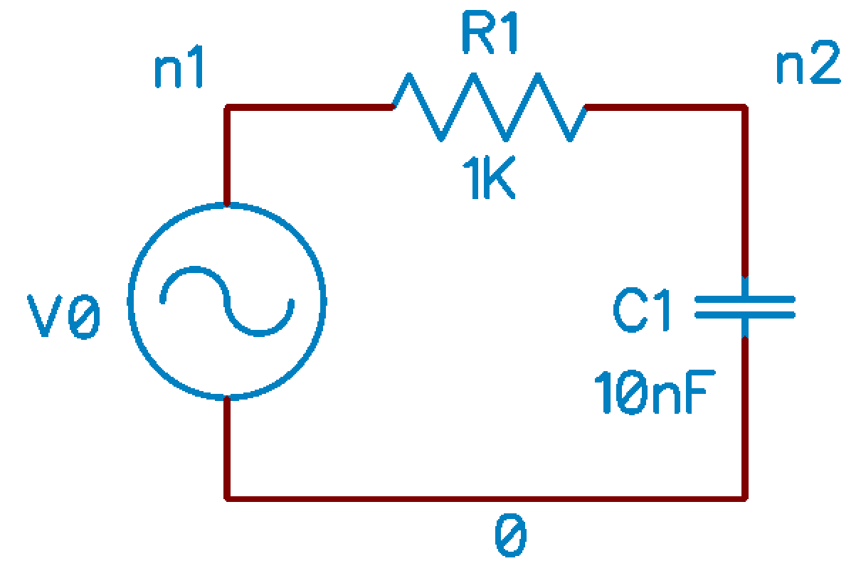
RC low pass filter

R1 n1 n2 1K
C1 n2 0 10nF
V0 n1 0 PULSE(-1 1 20US 0US 0US 100US 200US)
.end
Save the above circuit as ckt2-tran.cir. The voltage source is a periodic pulse train. The syntax for specifying a pulse train is
Vname N1 N2 PULSE(V1 V2 TD TR TF PW Period), where
V1 = initial voltage value
V2 = pulse voltage value
TD = delay before first change fron V1 to V2
TR = rise time
TF = fall time
PW = pulse width
Period = time period of the pulse train
Now, run the following analysis
ngspice -> source ckt2-tran.cir
ngspice -> tran 1us 1ms
ngspice -> plot v(n2)
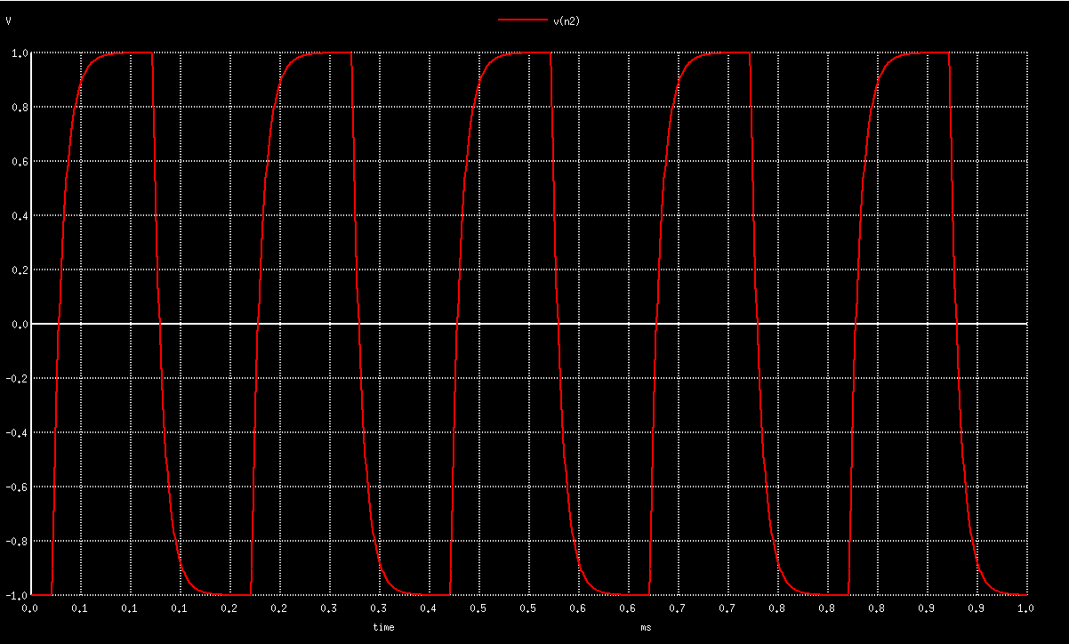
The syntax for running transient analysis is tran <tstep> <tstop> <tstart>
Finally, let us carry out AC analysis. The circuit for this analysis is the same as the one for transient analysis, except that the voltage source would be sinusoidal.
RC low pass filter

R1 n1 n2 1K
C1 n2 0 10nF
V0 n1 0 AC
.end
Save the above circuit as ckt2-ac.cir. Recall that AC analysis is all about varying the input voltage frequency over a range. Since we are dealing with linear circuits, the frequency of voltage and current at all nodes and loops in the circuit would have the same frequency (at steady state). SPICE provides a variety of ways of sweeping through a frequency range
- linear sweep
- decade sweep
- octate sweep
We will just look at linear sweep. The syntax for specifying linear sweep is
ac lin NumberOfPoints StartFreq EndFreq
As an example,
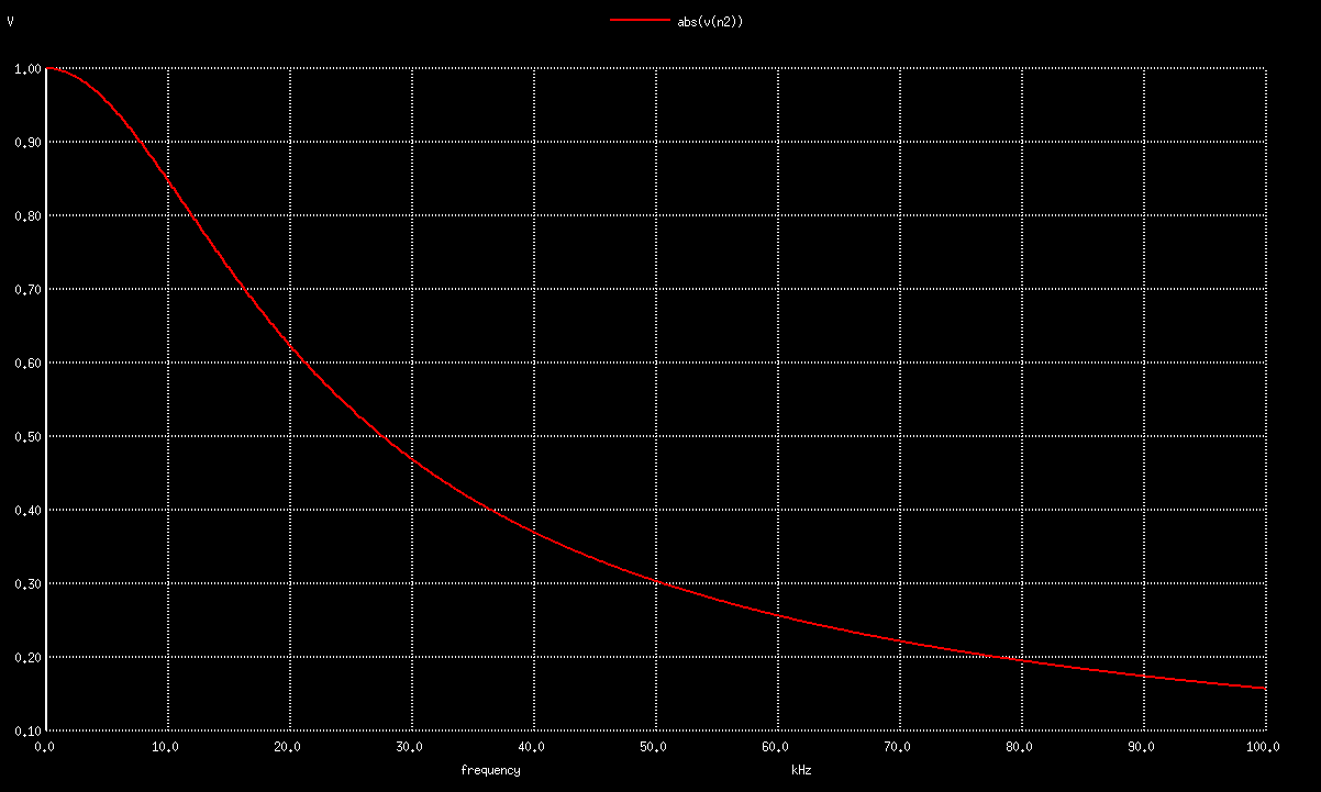
ngspice -> source ckt2-ac.cir
ngspice -> ac lin 1000 1 1k
ngspice -> plot abs(v(n2))
I would probably write a follow up tutorial on spice whenever I borrow some time from my workplace. Hopefully, this one was useful enough!
Tweetcomments powered by Disqus